The Data
Understanding the dataset through visualizations
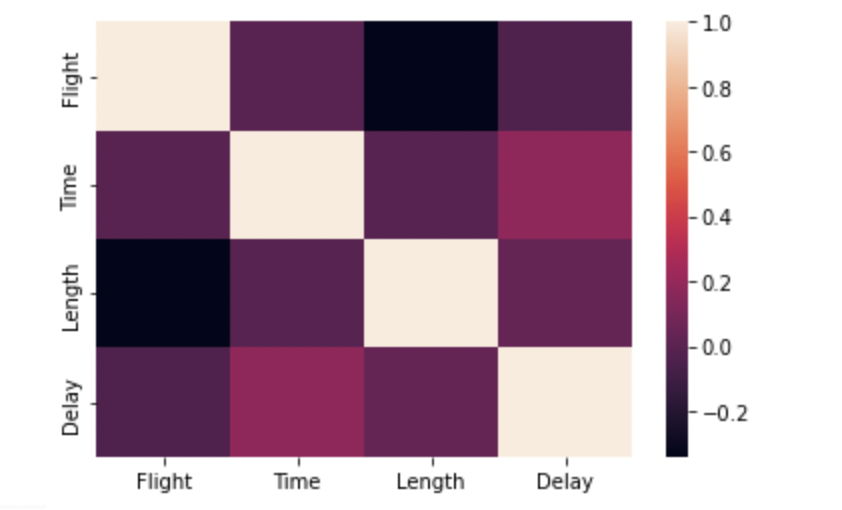
Heatmap
Relationships between features
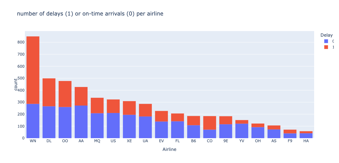
Airlines
Distribution of airlines in the dataset
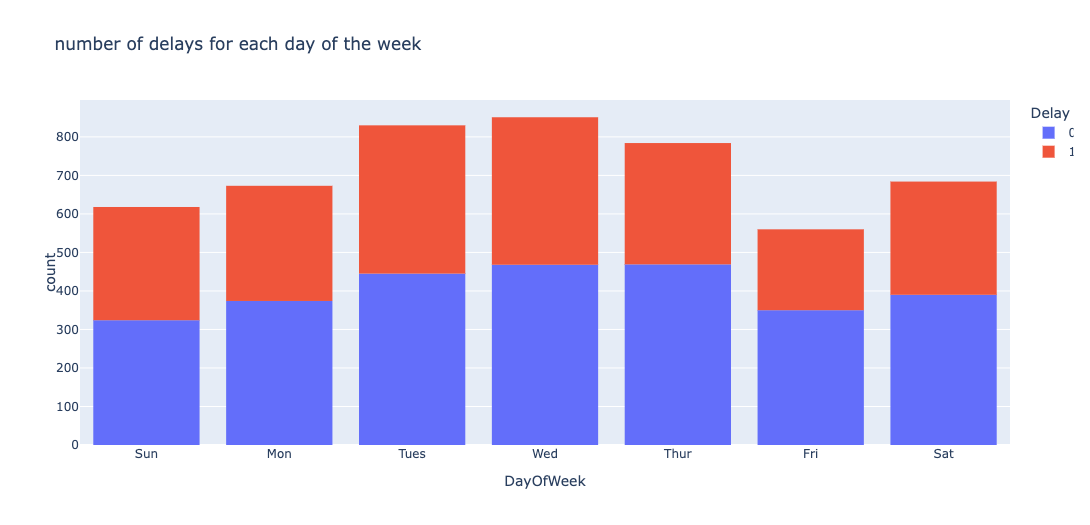
Day of Flight
Distribution of flights based on day of the week
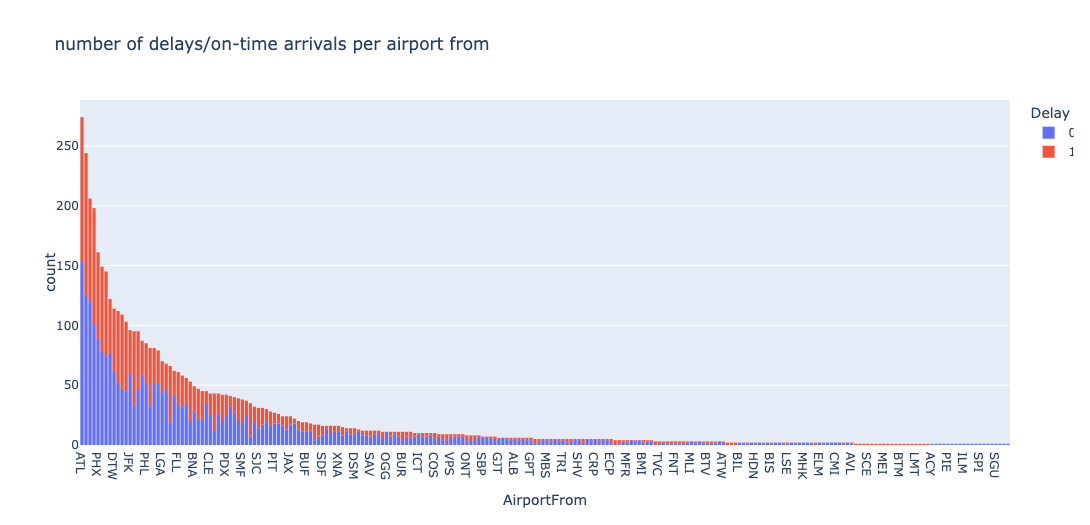
Source Airports
Distribution of on-time and delayed flights
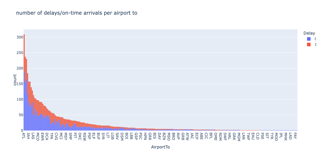
Destination Airports
Distribution of on-time and delayed flights
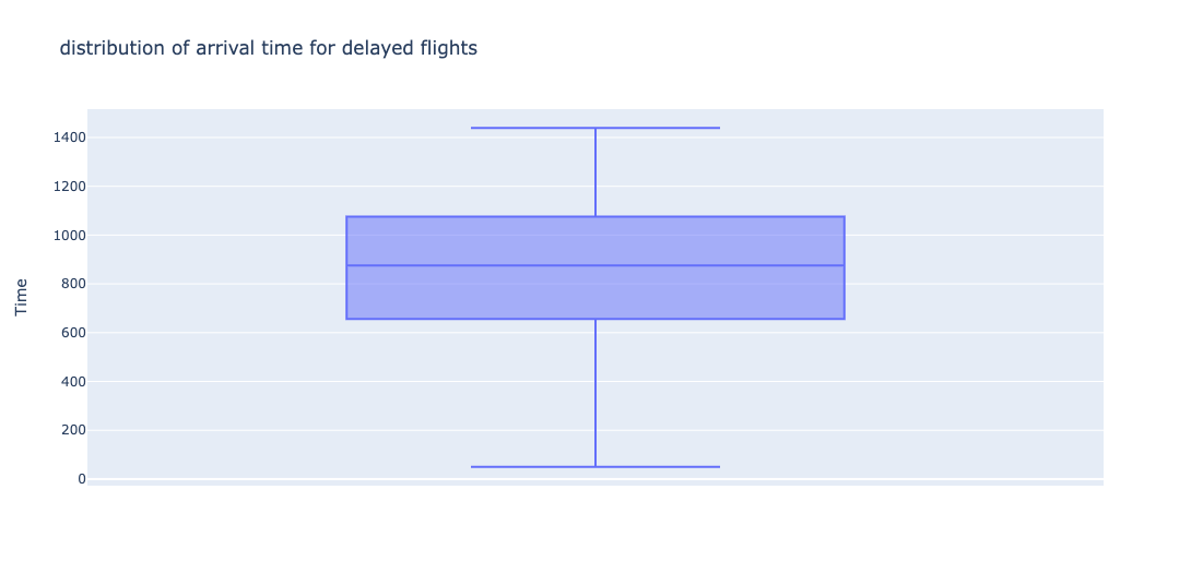
Arrival Times - Delay
Distribution of times when flight was delayed
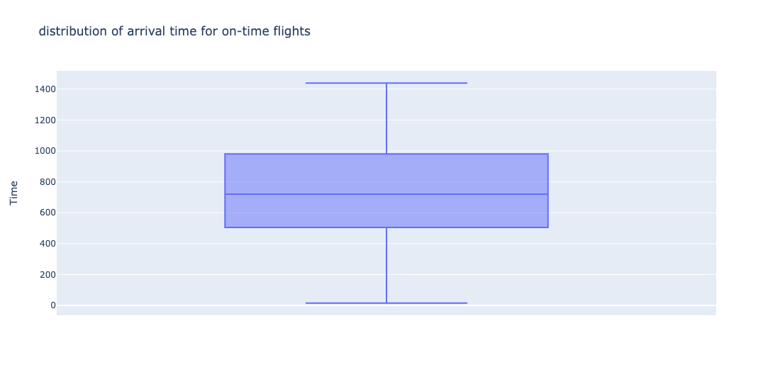
Arrival Times - On Time
Distribution of times when flight was on-time
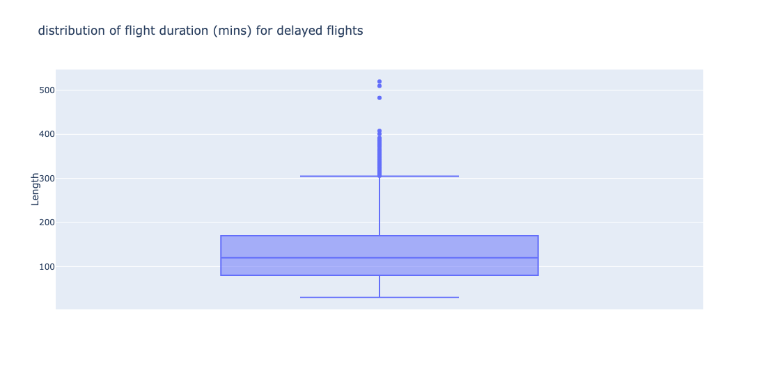
Flight Duration - Delay
Distribution of durations when flight was delayed
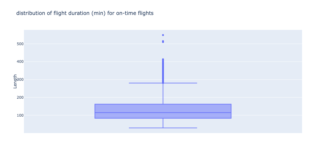
Flight Duration - On Time
Distribution of times when flight was on-time